Interdisciplinary Nonlinear Dynamics (438)

Take-Home Final

Due December 13, 12 noon

The final consists of 3 problems.

1. One-Dimensional Systems

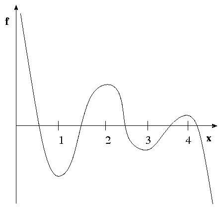
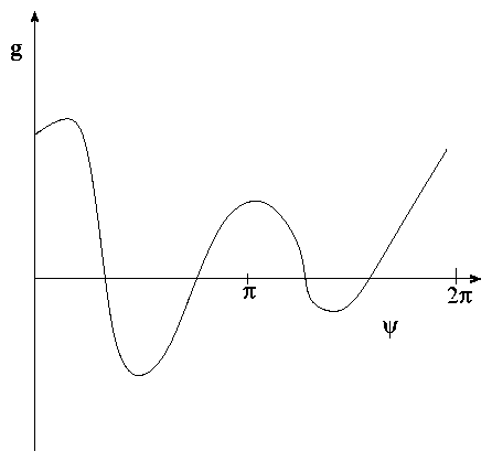
   Investigate the following two dynamical systems where f(x) and g(y) are sketched in the figure below,

   
   

   (I)       d dt x = l+ f(x), (II)       d dt y = l+ g(y)        with       g(y+2p) = g(y).

   Imagine an experiment in which you are scanning l to look for all stationary states of the system.

   1. For x(0) = 0 and y(0) = 0, respectivly, describe qualitatively the sequence of events that occur in (I) and (II) when the control parameter l is increased very slowly from large negative to large positive values and back again.
   2. Sketch x(t) and y(t), respectively.
   3. Do you observe hysteresis? How many different states are obtained performing this `experimental' protocol?
   4. Are there stationary states that are overlooked with this protocol?

2. Center-Manifold Reduction

   Consider the dynamical system

   
   

   d x dt = -x + my -y3-3xy2, (1) d y dt = 5x. (2)

   1. Perform a linear stability analysis of the basic solution (x = 0,y = 0) of (1,2). Determine also the eigenvectors associated with the two eigenvalues.
   2. Use the suspended system to perform a center manifold reduction of (1,2) for small m. To simplify the calculation identify a reflection-type symmetry of (1,2) and make use of it in the expansion. What type of bifurcation do you expect? When determining the center manifold, keep terms up to quintic order in the dependent variable and up to first order in m. Give the evolution equation on the center manifold to a corresponding order.
   3. Solve (1,2) numerically. Use suitable initial conditions to obtain good numerical approximations for the center manifold for m = 0.01. Then increase m in steps up to m = 0.3.
      - Does the agreement persist?
      - Plot the center manifold for representative values of m together with the analytical result and discuss the comparison.
      - Is the approximation much improved by keeping the fifth-order terms?
      - For the larger values of m, does the numerical simulation - without comparison with the analytically obtained center manifold - give a direct indication that the center-manifold reduction has broken down?
3. Nonlinear Evolution of Eckhaus Instability

   In class it was shown that within the Ginzburg-Landau equation long-wave deformations of steady patterns are described by the phase equation

   
   

   ¶T f = D(q) ¶X2 f (3)

   where the complex amplitude A of the pattern and the super-slow scales are given by

   
   

   A = R(X,T) eiqx+df(X,T)        X = dx        T = d2t       d << 1. (4)

   Here x and t are the slow space and time variables in the Ginzburg-Landau equation. When |q| is too large the diffusion coefficient D(q) is negative and the pattern is unstable. This linear instability is called the Eckhaus instability.

   For a weakly nonlinear description of the Eckhaus instability, which is valid for small D(q), (3) has to be extended to obtain the nonlinear phase diffusion equation

   
   

   ¶T f = ( D + E ¶X f)¶X2 f- G¶X4 f. (5)

   Here G > 0.

   1. Use (5) to perform a linear stability analysis of f = 0, which corresponds to a periodic pattern with wavenumber q. How does the onset of the instability depend on the system size L (assume periodic boundary conditions for f)?
   2. Perform a weakly nonlinear analysis of (5) using a yet slower time t to derive an amplitude equation for the amplitude A of the Fourier mode that destabilizes f = 0 first as D is decreased below 0 for a system size L. Identify the type of bifurcation that occurs when the periodic pattern becomes unstable.
   3. Within the Ginzburg-Landau description the pattern y([^x],[^t]) is given by

      
      

      y( ^ x   , ^ t   ) = e A(x,t)ei[^q]c[^x]+O(e2)+c.c. (6)

      Give an expression for the number of periods (i.e. number of maxima) of the pattern y when A is given by (4). For periodic boundary conditions one has f(X = 0,T) = f(L,T) for all T. Show that this implies that as long as the pattern is described by (5) the number of periods cannot change.

   4. Use the code from the class web site to solve the Swift-Hohenberg model

      
      

      ¶[^t] y = R y- (¶[^x]2+1)2y-y3 (7)

      numerically with periodic boundary conditions for R = 0.5. Start from a suitably chosen slightly perturbed periodic initial condition to illustrate what happens when the wavenumber of the pattern is in the Eckhaus-unstable regime. Show plots of y([^x],[^t]) for three times that are representative of the evolution arising from the Eckhaus instability.

   5. Comment on your results:
      How do the slightly perturbed periodic solutions evolve according to the amplitude equation that you have derived from (5) and how does this compare with the regime of validity of (5)?
      How do you reconcile the fact that within (5) the number of periods does not change with your numerical finding in the Swift-Hohenberg model?