The simulations solve equation
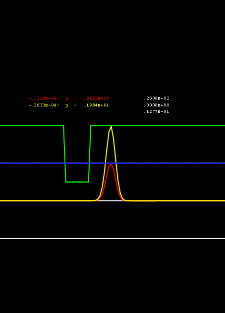
The density depends on space (green line in plot) and leads to the partial reflection of the pulse. The equations are solved with a (2,2) Leap-Frog scheme . The dissipation is added as a fourth-order spatial derivative with a small coefficient.
no dissipation: (in.1)
movie,
movie (gif)
Energy essentially constant, no blow-up
with dissipation without lag: (in.2) movie, movie (gif)
with dissipation with lag: (in.3) movie, movie (gif)
with larger dissipation with lag: (in.4) movie,
movie (gif)
blow-up in oscillatory mode.
Notes:
The stability limit is given by lambda=1-2*epsilon*g with g(pi)=8 and epsilon=0.03125 for disamp=0.000001 and lambda=0.25.
The energy is shown in the plots as the second number in the white column on the right.